Overview🔗
- Replicates Poletto et al.’s [58] setup and settings for Direct numerical simulation of turbulent channel flow up to Ret=590 [51]
- References: Van Driest (1956) [84], Smagorinsky (1963) [64], Kim et al. (1987) [28], Moser et al. (1999) [51], and Poletto et al. (2013) [58] (Synthetic turbulence inflow generator)
- See the resources section for additional data files
Flow physics:
- Internal flow
- Moderate Reynolds number
- Spanwise direction: Statistically homogeneous
- Streamwise and channel-height directions: Statistically developing
- Newtonian, single-phase, incompressible, non-reacting
Solver:
Tutorial case:
Physics and Numerics🔗
Physical domain:
- The case is a statistically-developing internal flow through parallel smooth
walls which are two characteristic-length apart.
- \(x\): Longitudinal direction (Mean-flow direction)
- \(y\): Vertical direction (Wall-normal direction)
- \(z\): Spanwise direction (Statistically homogeneous direction)
- \(O\): Origin at the left-bottom corner of the numerical domain
Physical modelling:
- Reynolds number based on friction velocity: \(\text{Re}_{u_\tau} = \vert \mathbf{U}_\tau \vert \delta / \nu_\text{fluid} = 395\) [-]
- (Estimated) Friction velocity: \(\mathbf{U}_\tau = (1.0, 0.0, 0.0)\), and \(\vert \mathbf{U}_\tau \vert = u_\tau = 1.0\) [m⋅s-1]
- Characteristic length (Channel half-height): \(\delta = 1.0\) [m]
- Kinematic viscosity of fluid: \(\nu_{\text{fluid}} \approx 0.002532\) [m2⋅s-1]
- Bulk velocity of flow: \(\mathbf{U}_b = (17.55, 0.00, 0.00)\) [m⋅s-1]
- Turbulence model: Large eddy simulation with the
Smagorinsky sub-filter scale model utilising the
van Driest wall-damping function. The
sub-filter scale model constants:
- \(C_k \approx 0.02655\)
- \(C_e = 1.048\)
- \(C_s \approx 0.065\)
- \(C_s = (C_k \{C_k/C_e\}^{0.5} )^{0.5}\)
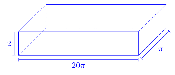
Numerical domain modelling:
- Shape: Rectangular prism
- Dimensions: \((x, y, z) = (20.0\pi, 2.0, \pi)\) [m]
- Sketch:
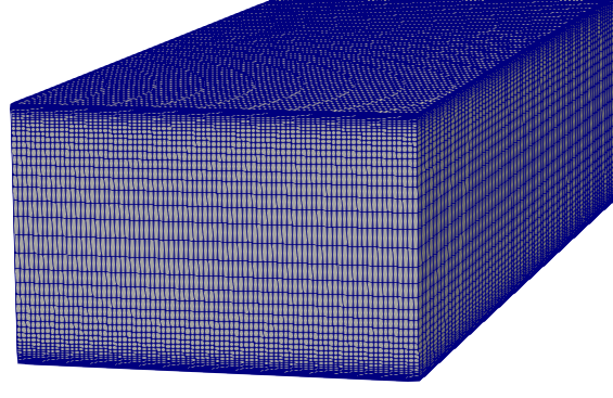
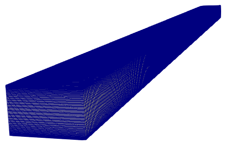
Spatial domain discretisation:
- Mesh type: Rectangular cuboid mesh
- Mesher: blockMesh
- Number of nodes, \(N\): \((N_x, N_y, N_z) = (500, 46, 82)\) [nodes]
- Spatial resolution \((\Delta)\) distribution:
- Uniform in \((x, z)\)-directions
- Stretched in \((y)\)-direction; clustered nearby walls
- Uniform mesh particulars:
- \(\Delta_x^+ = (\Delta_x u_\tau )/\nu_{\text{fluid}} \approx 49.6\) [-]
- \(\Delta_z^+ \approx 15.1\) [-]
- Wall-normal mesh particulars:
- Simple grading expansion ratio: 25.0 [-] (From top to bottom wall, the ratio is 0.04)
- First wall-normal node height: \(\Delta_y^+ \approx 1.1\)
- Mesh details:
 |
 |
Temporal domain discretisation:
- Time-step size: \(\Delta_t = 0.004\) [s]
- Estimated Courant-Friedrichs-Lewy (CFL) number based on \(\{ \overline{u_x} \}_{y^+ = 392} = 20.133\)[m⋅s-1]: CFL \(\approx 0.64\)
Equation discretisation:
Spatial derivatives and variables:
- Gradient: Gauss linear
- Divergence: Gauss
linear - Laplacian:
Gauss linear orthogonal - Surface-normal gradient: orthogonal
Temporal derivatives and variables:
-
ddtSchemes: backward
Numerical boundary conditions:
- Velocity, \(\mathbf{U}\)
| Patch | Condition | Value [m⋅s-1] |
|---|---|---|
| Inlet | turbulentDFSEMInlet | (17.55, 0.00, 0.00) |
| Outlet | inletOutlet | (0.0, 0.0, 0.0) |
| Sides (\(z\)-dir) | cyclic | - |
| Walls (\(y\)-dir) | fixedValue | (0.0, 0.0, 0.0) |
- Pressure,
p
| Patch | Condition | Value [m2⋅s-2] |
|---|---|---|
| Inlet | zeroGradient | - |
| Outlet | fixedValue | 0.0 |
| Sides (\(z\)-dir) | cyclic | - |
| Walls (\(y\)-dir) | zeroGradient | - |
- Turbulent kinematic viscosity,
nut(i.e. \(\nu_t\))
| Patch | Condition | Value [m2⋅s-1] |
|---|---|---|
| Inlet | calculated | - |
| Outlet | calculated | - |
| Sides (\(z\)-dir) | cyclic | - |
| Walls (\(y\)-dir) | zeroGradient | - |
Solution algorithms and solvers:
- Pressure-velocity: PISO
- Parallel decomposition of spatial domain and fields: scotch
- The bandwidth of the coefficient matrix is minimised by renumberMesh
- Linear solvers:
| Field | Linear Solver | Smoother | Relative Tolerance |
|---|---|---|---|
U |
smooth | GaussSeidel | 0.0 |
p |
GAMG | GaussSeidel | 0.0 |
nuTilda |
smooth | GaussSeidel | 0.0 |
Initialisation and sampling:
- Computation time for a single domain pass-through based on \({ \overline{U_x} }_{y^+ = 392} = 20.133\)) [m2⋅s-1] \(\approx 3.121\) [s]
- Initialisation pass-throughs = \(\approx 2.7\) [58]
- Sampling pass-throughs = \(\approx 24.5\) [58]
Results🔗
List of metrics:
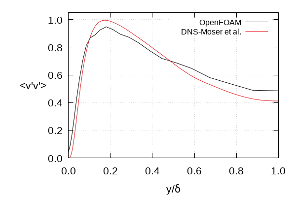
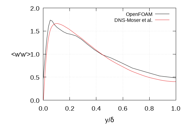
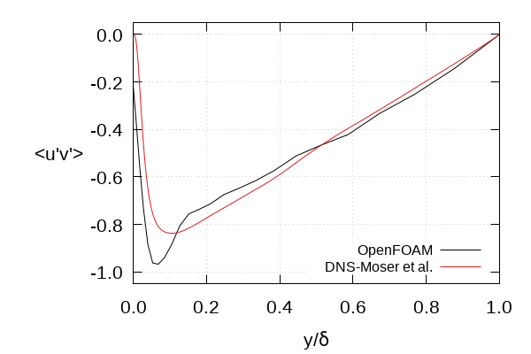
- Prescribed vs. reproduced Reynolds stress tensor components at inlet patch
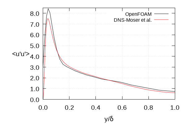
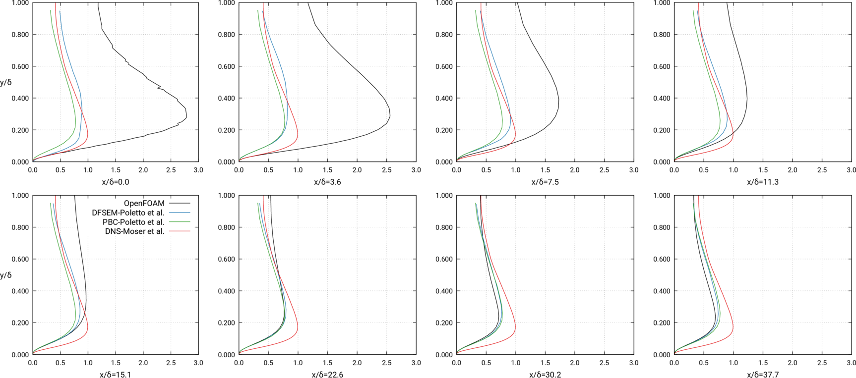
- \(\overline{u^\prime u^\prime}\) downstream development vs. \(x/ \delta\)
- \(\overline{v^\prime v^\prime}\) downstream development vs. \(x/ \delta\)
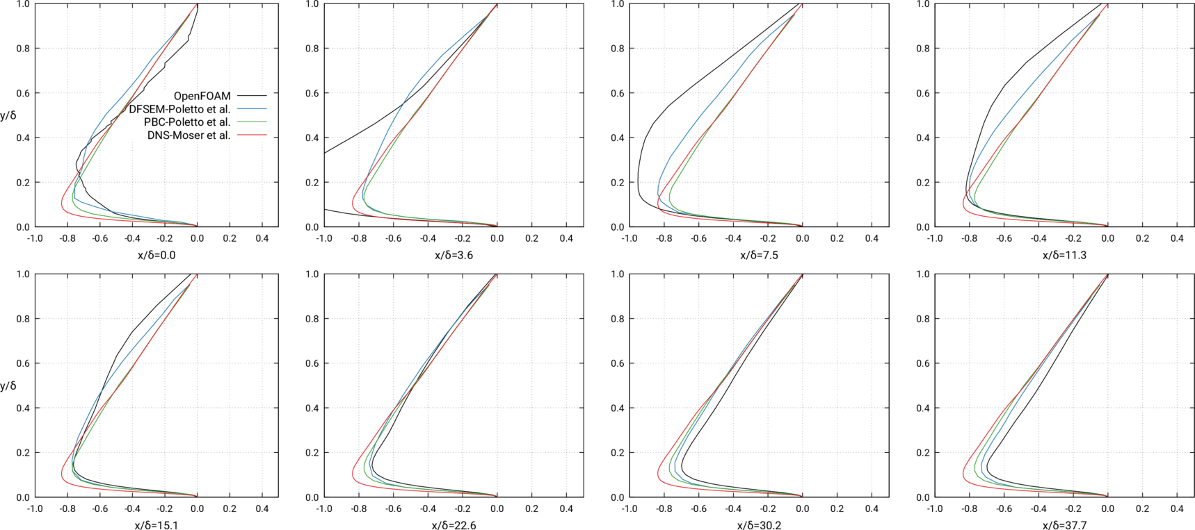
- \(\overline{u^\prime v^\prime}\) downstream development vs. \(x/ \delta\)
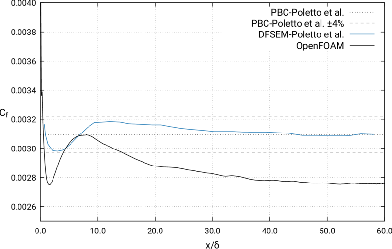
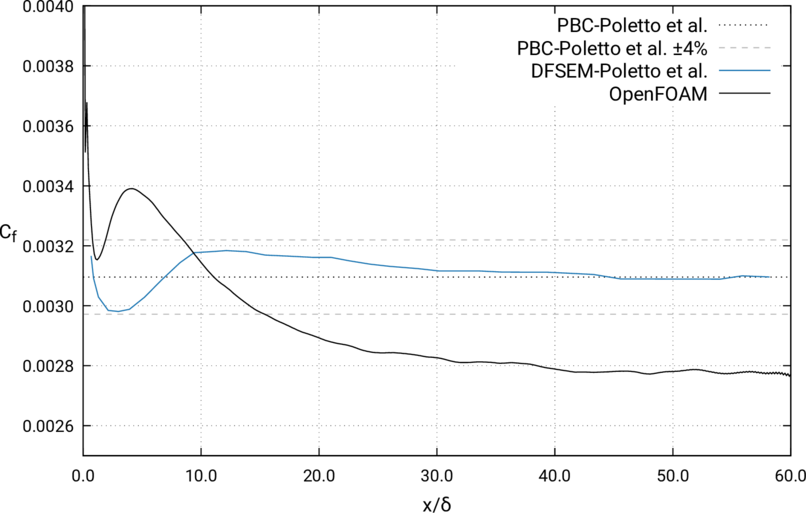
- Surface skin friction coefficient \(\mathrm{C}_f\) vs. \(x/ \delta\)
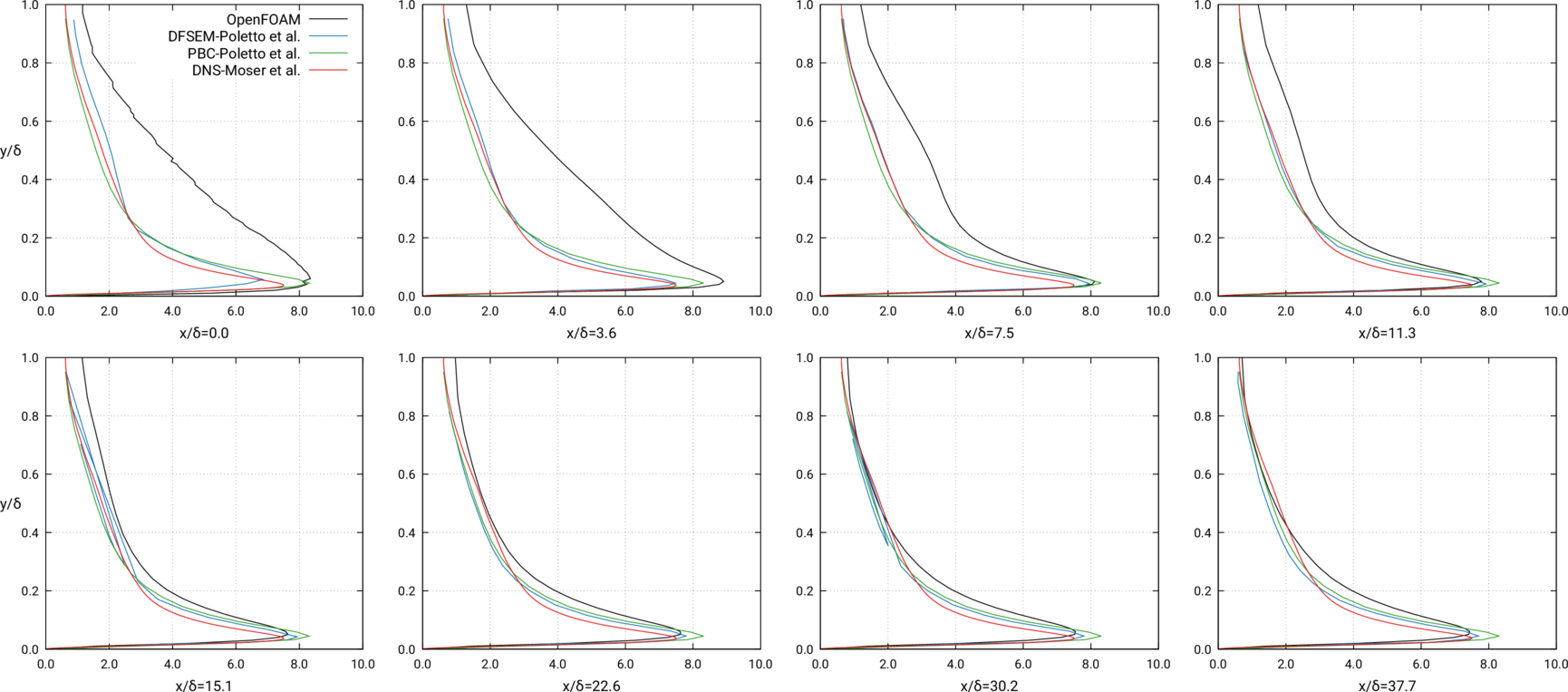
- Streamwise mean flow speed and Reynolds stress tensor components at uniform-interval downstream profiles
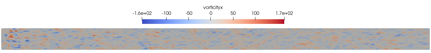
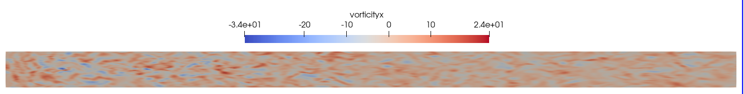
- Streamwise vorticity \(\omega_x\) at \(x/ \delta = 0.1\)
- Streamwise vorticity \(\omega_x\) at \(x/ \delta = 1.0\)
- Metrics are time and spanwise averaged
- \(< \cdot >\) is the time-averaging operator
 |
 |
 |
 |
 |
 |
 |
 |
 |
 |
 |
Resources🔗
Note: Links will take you to the University of Texas at Austin website
Datasets for verifications (plain text)🔗
Reynolds stress tensor profiles:
Mean velocity profiles:
Two-point velocity correlations (i.e. Auto- and cross-correlation functions):
