Overview🔗
- Solver: pimpleFoam
- Goals: Learn how to set up
-
Simulation with rotating mesh
- example: rotating fan in a room
Case files can be found here:
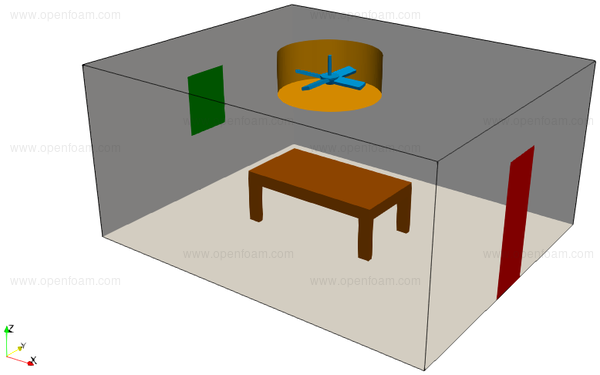
Geometry🔗
The geometry for this tutorial consists of
- room with
- door
- window (outlet)
- desk
- rotating fan
- cylinder defining
- rotating cells
- the interpolation surfaces between rotating and non-rotating cells
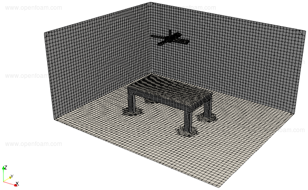
Mesh🔗
The mesh is created with snappyHexMesh using
STL surfaces located in the constant/triSurface directory.
surfaceFeatureExtract
The process begins by extracting features from the STL files (dictionary can be found in system/surfaceFeatureExtractDict).
blockMesh
This command creates an initial block structured mesh with our starting mesh resolution (dictionary can be found in system/blockMeshDict).
snappyHexMesh -overwrite
This command refines the initial mesh at the STL surfaces as well as the
extruded features (dictionary can be found in system/snappyHexMeshDict).
Layer addition is not utilized in this tutorial for simplicity purposes.
Usual snappyHexMesh settings are utilized for a coarse mesh here. One important
entry can be found in the refinementSurfaces sub-dictionary:
AMI
{
    level     (2 2);
    faceType  boundary;
    cellZone  rotatingZone;
    faceZone  rotatingZone;
    cellZoneInside inside;
}
This defines a cellZone called rotatingZone, which will later define the rotating cells. Additionally we define a boundary, which will be later used to define the interpolation faces between rotating and non-rotating regions.
renumberMesh -overwrite
This commands restructures the mesh for better calculation performance.
createPatch -overwrite
This command converts the boundary AMI to an arbitrary mesh interface (hence AMI), where during the simulation the interpolation of fields between rotating and non-rotating cells will take place (dictionary can be found in system/createPatchDict).
After these steps you can visualize your mesh in ParaView:
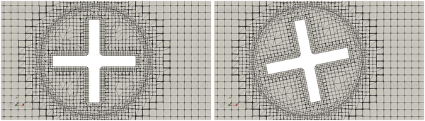
- Use higher refinement on AMI and fan for better mesh resolution.
- Use refinement region defined by AMI for uniform mesh resolution within rotating zone.
- This will however increase your calculation time.
Here you can see the rotating and non-rotating regions of the mesh:
Simulation🔗
Now we move from the folder mesh to the folder case.
Boundary conditions🔗
- Boundaries in the folder 0 are defined the following way:
- door: inlet
- outlet (window): outlet
- room: wall
- desk: wall
- fan: moving wall
- velocity U
- door: fixedValue with -0.1 m/s
- outlet (window): pressureInletOutletVelocity
- room: noSlip
- desk: noSlip
- fan: movingWallVelocity
- kinematic pressure p
- door:
fixedFluxPressure - outlet (window): fixedValue with atmospheric pressure at 0 Pa
- room:
fixedFluxPressure - desk:
fixedFluxPressure - fan:
fixedFluxPressure
- door:
- turbulent kinetic energy k
- door:
turbulentIntensityKineticEnergyInletwith 5% turbulence intensity - outlet (window): zeroGradient (alternative: inletOutlet
- room:
kqRWallFunction - desk:
kqRWallFunction - fan:
kqRWallFunction
- door:
- turbulent dissipation rate omega
- door:
turbulentMixingLengthFrequencyInletwith 1.2m mixing length - outlet (window): zeroGradient (alternative: inletOutlet)
- room:
omegaWallFunction - desk:
omegaWallFunction - fan:
omegaWallFunction
- door:
- turbulent kinematic viscosity nut
- door: zeroGradient
- outlet (window): zeroGradient (alternative: inletOutlet)
- room:
nutkWallFunction - desk:
nutkWallFunction - fan:
nutkWallFunction
Definition of mesh movement🔗
- Dictionary dynamicMeshDict can be found in constant.
- Important entries:
-
cellZone rotatingZone;- This was defined in snappyHexMeshDict to define the rotating cells. -
solidBodyMotionFunction rotatingMotion;- rotating mesh movement -
origin (-3 2 2.6);- origin of the axis of rotation of cells (can be anywhere on the rotation axis of the fan) -
axis (0 0 1);- direction of the rotation axis (here: z-direction) -
omega 10;- angular velocity of rotation in rad/s= (corresponds to ~95.5 rpm)
-
- For a realistic fan movement use
omega 20;
Additional dictionaries in constant🔗
- g - gravitational acceleration
- transportProperties - definition of kinematic viscosity
- turbulenceProperties - definition of turbulence model (here: kOmegaSST)
Simulation settings🔗
-
controlDict - runtime settings
- endTime: 1 s (approx. 0.64 s per revolution)
- writeInterval: 0.1 s
- maxCo: 1
- decomposeParDict - parallel setting
- fvSchemes - various discretisation schemes
- fvSolution - numeric settings (matrix solvers, tolerances, correctors)
Running the simulation🔗
The simulation employs the pimpleFoam application, in parallel.
decomposePar
With this command you divide your mesh and your fields onto multiple processors.
mpirun -np 4 pimpleFoam -parallel > log.pimpleFoam &
With this command you start your simulation on four cores. If you want to use a different number of cores you have to change the number (here: 4) to you choice. Also don’t forget to change the settings in system/decomposeParDict!
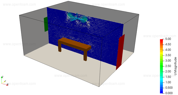
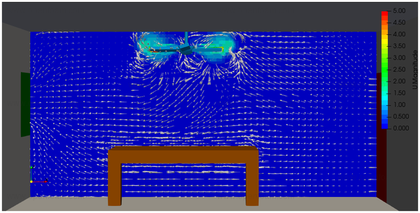
Results🔗
Here you see the flow after t = 0.64 s.
Velocity magnitude and vectors on a y-normal plane:
Close-up of velocity magnitude and vectors on a y-normal plane:
- For a more developed flow pattern run the simulation until 10-20s.
