Time scheme example
- Solver: scalarTransportFoam
- TODO: Repository link: TBA
Introduction
The test case comprises a 2-D box section, across which a uniform flow is applied. A passive scalar is introduced in a circular region at the start time, and transported across the domain. By looking at the profile of the scalar across the section, we can determine the characteristics of our time scheme selection.
Case set-up
The impact of the choice of time scheme is assessed by
varying the ddt scheme entry of the fvSchemes file:
ddtSchemes
{
    ddt(phi)        <time scheme>
}
Boundary conditions
Velocity boundary conditions
| Patch | Type | Value |
|---|---|---|
| left | fixedValue | (1,1,0) |
| right | zeroGradient | |
| top | zeroGradient | |
| bottom | fixedValue | (1,1,0) |
| frontAndBack | empty |
Scalar boundary conditions
| Patch | Type | Value |
|---|---|---|
| left | fixedValue | 0 |
| right | zeroGradient | |
| top | zeroGradient | |
| bottom | fixedValue | 0 |
| frontAndBack | empty |

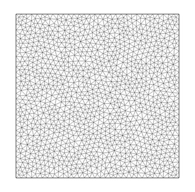
Mesh
Results
Euler results


backward results


Crank-Nicolson results


