Welcome to the OpenFOAM® quickstart guide!
This guide provides a simplified step-by-step overview to help you quickly get started with the installation, setup, and basic usage of OpenFOAM®, a powerful free/open-source computational fluid dynamics (CFD) software.
OpenFOAM® Installation🔗
OpenFOAM® is easily accessible on a wide range of operating systems, including Linux distributions, Microsoft Windows, and macOS. You can conveniently obtain OpenFOAM® in the form of precompiled packages or as source code that you can build yourself.
In this guide, we will install the precompiled package of the latest OpenFOAM® version on Microsoft Windows 10 Enterprise operating system.
Download the package of the latest OpenFOAM® version by simply clicking the link below (Please ensure that you have at least 300MB of available storage space on your hard disk):
Link to OpenFOAM-windows-mingw.exe
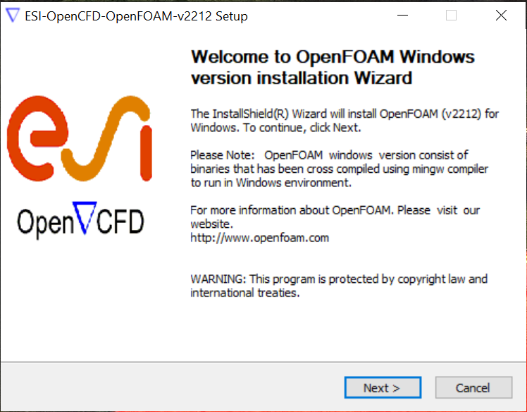
The package is an executable. Run this executable to open the installation wizard, and simply follow the wizard’s installation instructions specific to your system. A typical view of the wizard is shown below (Please ensure that you have enough available storage space on your hard disk):
You may also need to install Microsoft MPI (MS-MPI). Similary, download
the following package (i.e. msmpisetup.exe), and follow its installation
wizard:
Upon completion of the above steps, an icon will be created on your desktop.
Double-click this icon to launch a terminal window. Running this icon will load
the OpenFOAM® environment. Verify the contents of OpenFOAM® in a
terminal as follows ($ is the command prompt, indicating that the
terminal is ready to
accept a command.):
$ ls -p
OpenFOAM/

$ cd $WM_PROJECT_DIR

$ ls -p
bin/  COPYING  etc/  etc-mingw  META-INFO  platforms/  README.md  ThirdParty/  tutorials/
Problem Setup🔗
The problem setup is derived from the experiment conducted by Pitz and Daily (1983).
The setup involves a steady simulation of a non-reacting, single-phase, Newtonian, incompressible fluid flow, which comprises a range of intricate turbulence phenomena such as flow detachment/reattachment and formation of recirculation zones.
You can browse the problem setup:
$ cd $FOAM_TUTORIALS/incompressible/simpleFoam/pitzDaily/

$ ls -p
0/  constant/  system/

$ ls -p system/
blockMeshDict  controlDict  fvSchemes  fvSolution  streamlines

$ ls -p constant/
transportProperties  turbulenceProperties

$ ls -p 0/
epsilon  k  p  U
In OpenFOAM®, simulation settings are customised using text files. Each parameter in these files follows a straightforward key-value pair format. However, it is important to note that each file has its own unique set of mandatory and optional keywords. The location and content of these files vary depending on the chosen solver application, simulation setup, and the specific aspects you wish to modify. Therefore, it is necessary to familiarize yourself with the structure and significance of these keywords in relevant files.
Pre-process🔗
Pre-processing involves the typical preparation steps of a CFD problem setup.
To carry out these steps, it is necessary to be familiar first with the typical directory structure of an OpenFOAM® setup and the meaning of these directories.
An OpenFOAM® simulation generally consists of the following three directories:
-
0: (zero directory) contains field initial/boundary conditions at timestep (or iteration) zero. Note that fields are typically named according to their mathematical representation, e.g.ufor velocity,pfor pressure,Tfor temperature etc. -
constant: contains files that define the geometric and physical properties of the simulation. -
system: contains files that define the settings of the simulation applications and tools.
Physical domain🔗
In OpenFOAM®, there are multiple ways to provide the physical domain specifications for a simulation. These include:
- Geometry import: OpenFOAM® supports the import of geometry from
external sources in formats such as
STL,STEP, orIGES, to name a few. - Geometry definition: OpenFOAM® allows manual definition of the physical domain within itself.
- Mesh generation: OpenFOAM® provides native meshing tools including blockMesh, snappyHexMesh, and mesh converters to generate meshes that represent the physical domain.
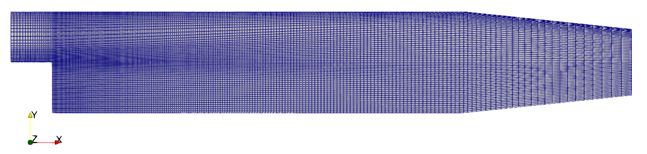
In this example, we generate the physical domain alongside the mesh using the blockMesh utility. The physical domain includes a narrow inlet passage, a backward-facing step, and a converging section, as shown in the side view below:

Physical properties🔗
In this example, we consider a simple non-reacting, single-phase, Newtonian, incompressible fluid flow, with the following physical properties:
| Metrics | Values |
|---|---|
| Fluid kinematic viscosity, \(\nu\) | \(1e\text{-}5\,[\mathrm{m}^2\text{/}\mathrm{s}]\) |
In OpenFOAM®, the type of fluid and the value of the fluid kinematic
viscosity are set using the transportProperties file located in the
constant directory.
$ cat constant/transportProperties

[...]

transportModel  Newtonian;
nu              1e-05;

[...]
Spatial domain discretisation🔗
In this example, we generate the spatial domain discretisation, also known
as the mesh, using the blockMesh utility configured by
the blockMeshDict file in the system directory.
You can skim through the content of this file via (for further information, please see blockMesh):
$ cat system/blockMeshDict
The side view of the generated mesh is illustrated below:
In OpenFOAM®, the spatial domain discretization is typically performed using one of three methods, depending on the complexity of the physical domain and the desired mesh characteristics:
- blockMesh: built-in mesh generation tool in OpenFOAM® providing a simple and intuitive way to generate structured meshes for simple geometries.
- snappyHexMesh: powerful built-in mesh generation tool in OpenFOAM® used for generating high-quality, unstructured meshes. It can handle complex geometries and supports various meshing strategies, such as refinement regions and boundary layer additions.
- Mesh conversion: OpenFOAM® supports the import of meshes generated by
various external mesh generators using tools like
fluentMeshToFoam.
Temporal domain discretisation🔗
In this example, the temporal domain discretization, i.e. the division of the simulation time into discrete steps, is steady state.
In OpenFOAM®, the temporal domain discretization is set in the
controlDict file located in the system directory.
The following key-value pairs in the controlDict file allow users to configure the temporal behaviour of the simulation:
$ cat system/controlDict

[...]

startFrom       startTime;
startTime       0;
stopAt          endTime;
endTime         2000;
deltaT          1;
adjustTimeStep  off;

[...]
OpenFOAM® provides several methods to handle the temporal discretization, allowing users to control the time advancement and accuracy of their simulations. Here are the main methods for generating the temporal domain discretization in OpenFOAM®:
- Steady-state simulations
- Explicit time stepping
- Implicit time stepping
- Adaptive time stepping
Equation discretisation🔗
In OpenFOAM®, the equation discretization refers to the numerical approximation of the governing equations that describe fluid flow or other physical phenomena. OpenFOAM® provides a wide range of discretization schemes that can be used to discretize the equations and solve them numerically.
The selection of discretization schemes is usually defined for each equation
field and equation type in the fvSchemes file found in the
system directory.
Within the fvSchemes file, you will find configurations for discretization schemes applied to gradient, divergence, Laplacian, and other terms in the governing equations.
For instance, you can examine the settings for time and gradient schemes within the fvSchemes file, as shown below:
$ cat system/fvSchemes

[...]

ddtSchemes
{
    default         steadyState;
}

gradSchemes
{
    default         Gauss linear;
}

[...]
Initial/boundary conditions🔗
In this example, the initial and boundary conditions of the governing equations at geometric boundaries are set as follows:
| Property | Inlet | Outlet | Walls | Internal |
|---|---|---|---|---|
| $$\text{Velocity}, \u \, [\text{m/s}]$$ | $$(10, 0, 0)$$ | $$\grad \u = \tensor{0}$$ | $$(0, 0, 0)$$ | $$(0, 0, 0)$$ |
| $$\text{Pressure}, p \, [\mathrm{m}^2\text{/}\mathrm{s}^2]$$ | $$\grad p = \vec{0}$$ | $$0$$ | $$\grad p = \vec{0}$$ | $$0$$ |
| $$\text{Turbulent kinetic energy}, k \, [\mathrm{m}^2\text{/}\mathrm{s}^2]$$ | $$0.375$$ | $$\grad k = \vec{0}$$ | $$\text{wall function}$$ | $$0.375$$ |
| $$\text{Turbulent kinetic energy dissipation rate}, \epsilon \, [\mathrm{m}^2\text{/}\mathrm{s}^3]$$ | $$14.855$$ | $$\grad \epsilon = \vec{0}$$ | $$\text{wall function}$$ | $$14.855$$ |
In OpenFOAM®, the initial and boundary conditions are specified using
field files located within time directories for each field variable, such as
velocity. The initial conditions are applied to the entire domain volume,
while the boundary conditions are specified on the boundaries of the domain,
which are divided into numerical patches.
For example, the initial condition for pressure field (\(p\)) is specified in
the p file within the 0 directory as shown below:
$ cat 0/p

[...]

internalField   uniform 0;

[...]
Similarly, as an example, the boundary condition for velocity field (\(\u\)) at
inlet patch is set in the U file within the 0 directory in the following
manner:
$ cat 0/U

[...]

boundaryField
{
    inlet
    {
        type            fixedValue;
        value           uniform (10 0 0);
    }

[...]
Pressure-velocity coupling algorithm🔗
In this example, the choice of the pressure-velocity coupling algorithm is the SIMPLE algorithm. The corresponding solver application in OpenFOAM® is called simpleFoam.
The settings for the SIMPLE algorithm can be specified in a sub-dictionary within
the fvSolution file, which is located in the system
directory:
$ cat system/fvSolution

[...]

SIMPLE
{
    nNonOrthogonalCorrectors 0;
    consistent      yes;           // SIMPLEC

    residualControl                // Additional control on simulation
    {
        p               1e-2;
        U               1e-3;
        "(k|epsilon)"   1e-3;
    }
}

[...]
Note that OpenFOAM® provides three pressure-velocity coupling algorithms:
- SIMPLE: Semi-Implicit Method for Pressure-Linked Equations
- PISO: Pressure Implicit with Splitting of Operators
- PIMPLE: Combination of PISO and SIMPLE
Linear solvers🔗
OpenFOAM® offers a range of linear solvers, including iterative solvers like
GAMG, PCG, and
PBiCG, as well as interfaces to external solvers, e.g.
PETSc. The choice of linear solvers and their parameters depends on various
factors such as the problem characteristics, size of the linear system, and
desired computational efficiency. OpenFOAM® provides extensive options for
fine-tuning its solver suites.
In OpenFOAM®, the settings for linear solvers are typically defined in the
fvSolution file located in the system directory.
For instance, the linear solver settings for the pressure field (\(p\)) are specified with the corresponding smoother and convergence parameters, as demonstrated below:
$ cat system/fvSolution

[...]

p
{
    solver          GAMG;
    smoother        GaussSeidel;
    tolerance       1e-06;
    relTol          0.1;
}

[...]
Case control🔗
In OpenFOAM®, the main case controls can be set in the
controlDict file
within the system directory. The controlDict file is
a key configuration file that allows you to control various aspects of the
simulation and specify case-specific settings such as:
- Time/Iteration control
- Output control
- Runtime control
- Function-object control
- Debug control
- Optimisation control
- External library control
The following shows a typical set of key-value pairs available in the controlDict:
$ cat system/controlDict

[...]

application     simpleFoam;         // name of solver application

startFrom       startTime;          <--
startTime       0;                  //
stopAt          endTime;            // Time/Iteration control
endTime         2000;               //
deltaT          1;                  -->

writeControl    timeStep;           <--
writeInterval   100;                //
purgeWrite      0;                  //
writeFormat     ascii;              // Output control
writePrecision  6;                  //
writeCompression off;               //
timeFormat      general;            //
timePrecision   6;                  -->

runTimeModifiable true;             // Runtime modifications

functions                           <--
{                                   //
    #includeFunc streamlines        // Function objects
    #include "streamlines"          //
}                                   -->

DebugSwitches                       <--
{                                   //
    SolverPerformance   0;          // Debug control
}                                   -->

OptimisationSwitches                <--
{                                   //
    writeNowSignal  12;             // Optimisation control
}                                   -->

libs                                <--
(                                   //
    externalLibraryName             // External library control
);                                  -->

[...]
Process🔗
To run this case, you can simply execute two consecutive commands.
First, the mesh is generated using the blockMesh utility. Run the utility with the following command (the execution should take a few seconds):
$ blockMesh
This command will display various utility messages and generate the mesh in the
constant/polyMesh directory. You can verify the mesh generation by checking
the contents of the directory using the command:
$ ls -p constant/polyMesh/
boundary  faces  neighbour  owner  points
If you need to make changes to the blockMeshDict settings or redirect the
utility’s output to a log file, you can rerun the
blockMesh using the command:
$ blockMesh >& log.blockMesh
You can also use the internal runner functions available in OpenFOAM®
(e.g. runApplication):
$ source ${WM_PROJECT_DIR:?}/bin/tools/RunFunctions

$ runApplication blockMesh
The next and final step is to run the solver application by executing the following command (the execution should take a few seconds):
$ simpleFoam >& log.simpleFoam
Running this command will run the simulation and print valuable information into the log file. This information includes updates on the convergence of the linear solvers, progress in simulation iterations, and details about function objects, among others.
Upon completion of the simulation, you will notice that OpenFOAM® has created new time directories containing solutions specific to each time step, post-processing data generated by function objects, and log files:
$ ls -p
0/  100/  200/  282/  constant/  log.blockMesh  log.simpleFoam  postProcessing/  system/
Post-process🔗
Once the simulation has been completed, the next step is post-processing the results to extract meaningful information and visualize the data. OpenFOAM® provides many powerful tools for post-processing that can be executed during runtime and/or after the simulation, e.g. postProcess utility.
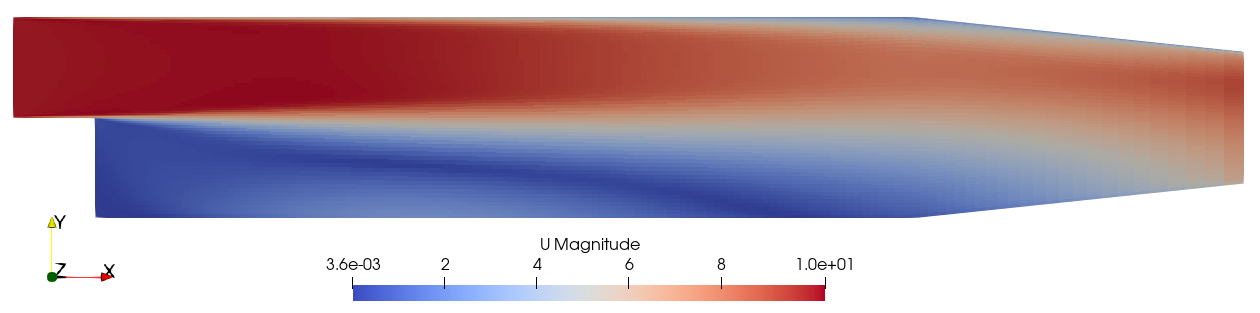
You can visualise the simulation results by an external visualiation toolkit. One of the most commonly used tools for field visualization is ParaView, an open-source visualization software that integrates well with OpenFOAM®.
An example visualisation of the velocity magnitude field at the last iteration step using ParaView can be seen below: